Proposed Title :
Low Power and Area Efficient Computation and Energy Reduction Technique for HEVC Discrete Cosine Transform
Improvement of this Project:
The proposed architecture was implemented 2D DCT Transform unit, with interchanged the co-efficient between column and row process, without Transpose memory and all TU sizes is implemented in Verilog HDL, and synthesized in Xilinx FPGA
Software implementation:
- Modelsim
- Xilinx 14.2
Proposed System:
In the proposed system, to design the DCT architecture for HEVC without transposed memory. Because of the datapath coefficient matrix for row and column are transpose each other for 16×16, 8×8 and 4×4 datapath. In the proposed system to use the following components,1)forward transform input splitter, 2)16×16, 8×8 and 4×4 datapath and butterfly structure for both column and row processing3) 32×32,16×16,8×8 and 4×4 butterfly design. DCT is split into two modules. That are work in the 1D DCT format.1) column butterfly structure and 2) row butterfly structure. In butterfly design to is used to change the input data into frequency domain. But in the different between the column and row process is butterfly design in row structure butterfly output is divided by 2.
The datapath is used to perform the matrix multiplication process. In the matrix multiplication first multiplies the one of the matrix column data to another matrix row data then addition process for thus values to get the first value of row output data. In matrix multiplication one of the matrixes is input data matrix and another one is coefficient matrix for both column and row. The coefficient for thus datapaths is generated based on the basic DCT equation. The outputs of the 2D DCT architecture is compressed images of input images. Input splitter is used to select the proper DCT inputs for each TU size. For example to use 32*32 DCT means to select the inputs 32 data sequences input signal. Its means this is act as a serial to parallel conversion. The output of the forward transform input splitter is 32 data in after 32 clock cycle.
Data = { 1,2,3,4,5,6,7,8,9,10,11,12,13,14,15,16,17,18….}
Output= {1,2,3,4,5,6,7,8,9,10,11,12,13,14,15,….32},{33,34,35,36,….. 64},{65,….
” Thanks for Visit this project Pages – Buy It Soon “
A Computation and Energy Reduction Technique for HEVC Discrete Cosine Transform
“Buy VLSI Projects On On-Line”
Terms & Conditions:
- Customer are advice to watch the project video file output, before the payment to test the requirement, correction will be applicable.
- After payment, if any correction in the Project is accepted, but requirement changes is applicable with updated charges based upon the requirement.
- After payment the student having doubts, correction, software error, hardware errors, coding doubts are accepted.
- Online support will not be given more than 3 times.
- On first time explanations we can provide completely with video file support, other 2 we can provide doubt clarifications only.
- If any Issue on Software license / System Error we can support and rectify that within end of the day.
- Extra Charges For duplicate bill copy. Bill must be paid in full, No part payment will be accepted.
- After payment, to must send the payment receipt to our email id.
- Powered by NXFEE INNOVATION, Pondicherry.
Payment Method :
- Pay Add to Cart Method on this Page
- Deposit Cash/Cheque on our a/c.
- Pay Google Pay/Phone Pay : +91 9789443203
- Send Cheque through courier
- Visit our office directly
- Pay using Paypal : Click here to get NXFEE-PayPal link